たれぱんのびぼーろく

わたしの備忘録、生物学とプログラミングが多いかも

sys.float_info.minと配列代入の罠 - numpy float32

sys.float_info.min (とても小さい値) を代入しても何故か0.になる。logが死ぬ。
データ型を疎かにしてたらハマった.

再現コード

float_array = numpy.array([1., 2.,], dtype=np.float32)
tiny = sys.float_info.min
print(float_array)
# [1. 2.]

float_array[1] = tiny
print(float_array)
# [1. 0.]
# 0. …だと…!?

match = float_array[1] == tiny
print(f"float_array[1] == tiny: {match} ({float_array[1]} vs {tiny})")
# float_array[1] == tiny: False (0.0 vs 2.2250738585072014e-308)

原因

Pythonにはfloatの更なる区分 (FP32/floatとFP64/doubleとか) がない.
でもnumpyには浮動小数点精度が複数ある.
sys.float_info.minは内部で利用されてくる精度の値を出してくるけど、numpyは指定したdtypeで値を受け入れる.
float64の最小値をfloat32で表現すると0.なので、0代入が発生しちゃう.

よくあるシチュエーション

外部ライブラリがnumpy arrayを返してくるが、そのデータ型を意識していない.
その状態でarrayの一部をsys.float_info.minで上書きしようとしたのに、なぜか0.になる.
結果logが死ぬ.

解決策

numpyを使うなら、使ってるdtypeの最小値を使えばいい.

float_array = numpy.array([1., 2.,], dtype=np.float32)

false_tiny = sys.float_info.min
true_tiny = np.finfo(float_array.dtype).tiny
print(false_tiny) # 2.2250738585072014e-308
print(true_tiny)  # 1.1754944e-38

float_array[1] = true_tiny
print(float_array) # [1.0000000e+00 1.1754944e-38]
match = float_array[1] == true_tiny
print(f"float_array[1] == tiny: {match} ({float_array[1]} vs {true_tiny})")
# float_array[1] == tiny: True (1.1754943508222875e-38 vs 1.1754943508222875e-38)

その他tips

Pythonのfloat精度は実行環境によるっぽい.
これが原因で「別の環境に持ってったら壊れた!?」とかはありうる.

librosaとscipyでFFTをマッチさせる

背景

librosaはSTFTがとっても便利。
プリミティブにFFTをしようと思ったらscipy.fft.rfftになる.
この2つ、同じ動作するのだろうか?

動作

デフォルト動作だと違う動きをする.
以下が同じ動作をする

librosa.stft(x_full, n_fft=n_fft, window="boxcar", center=False)
scipy.fft.rfft(x)

librosa.stftは実数信号のみを受け付け、デフォルトで窓関数を適用、windowはcenteringする.
なので窓関数をboxcar/矩形波にして事実上の窓無し、centering OFFにする.

scipy.fft.rfftはただただ入力全長にDFT掛けるだけ.

検証

import numpy as np
import scipy.fft
import matplotlib.pyplot as plt
import librosa

# Settings
n_fft = 512
input_r = np.linspace(0., 1., n_fft)

# Conversion
spec_mag_rfft = np.abs(scipy.fft.rfft(input_r))
spec_mag_stft = np.abs(librosa.stft(input_r, n_fft=n_fft, window="boxcar", center=False))[:, 0]
spec_mag_stft_hann = np.abs(librosa.stft(input_r, n_fft=n_fft, center=False))[:, 0]

# Plot
freq = scipy.fft.rfftfreq(n_fft)

plt.subplot(2, 1, 1)
plt.title("Frequency domain")
plt.plot(freq, spec_mag_rfft)
plt.plot(freq, spec_mag_stft)

plt.subplot(2, 1, 2)
plt.title("Diff")
plt.plot(freq, spec_mag_rfft - spec_mag_stft)
print(f"maximum diff: {np.max(np.abs(spec_mag_rfft - spec_mag_stft))}") # 0.
print(f"maximum diff (window): {np.max(np.abs(spec_mag_rfft - spec_mag_stft_hann))}") # very big

IFFT

も同じ感じ.

import sys
import numpy as np
import scipy.fft
import matplotlib.pyplot as plt
import librosa

# Settings
n_fft = 512
input_log_mag_spec = 20. * np.log(np.abs(scipy.fft.rfft(np.linspace(0., 1., n_fft)))  + sys.float_info.min)

# Conversion
ceps_irfft = np.abs(scipy.fft.irfft(input_log_mag_spec))
ceps_istft = np.abs(librosa.istft(input_log_mag_spec.reshape((input_log_mag_spec.shape[0], 1)), window="boxcar", center=False))

# Plot
freq = range(0, n_fft)

plt.subplot(2, 1, 1)
plt.title("Cefrency domain")
plt.plot(freq, ceps_irfft)
plt.plot(freq, ceps_istft)

plt.subplot(2, 1, 2)
plt.title("Diff")
plt.plot(freq, ceps_irfft - ceps_istft)
print(f"maximum diff: {np.max(np.abs(ceps_irfft - ceps_istft))}") # 0.

離散信号のメル化が抱える難点

  1. 必ず周波数分解能が落ちる

なんで?

離散の周波数成分1つは、それ以上分割できないquantumだから。

高周波成分の分解能を粗くすれば低周波を逆に精密に記述できる!…わけではない.
離散信号はもう周波数の離散化/量子化がなされてるので、post-hocに取り出せない.
連続信号のサンプリング (離散化) 時になら工夫のしようがあるかもだけど、離散信号へのメル化時には原理的に手が出ない.

なので離散信号のメル化 = 周波数weight付き情報圧縮
DNNでlinearなspectrogramが好まれる一因はたぶんこれ (empirically 圧縮率の良い特徴量、としてメル化する例も多いけどね)

おまけ: 連続信号のメル化

周波数表現上の関数 A=log(f) で表現される連続信号があるとする.
離散化bin数がNに固定される条件下で離散化せよ

メル尺度上で等間隔にbinを切れば、linear尺度で切った時より低周波帯で分解能がよくなる. なのでメル化はとても有用.

ビット分割

n-bitの整数を整数の組み合わせで表現する方法.
上位ビット/下位ビットみたいなやつ.

表現

6bit == 26 == 0~63
これを上位3bitと下位3bitに分割し、そのペアで表現する.
(3bit, 3bit) == (23, 23) == (0~8, 0~8)

変換法

上位decimal = valuedecial // 2nbit/2
下位decimal = valuedecial % 2nbit/2

例: 34
34 // 8 = 4, 34 % 8 = 2 => (4, 2) == 100/010 == 34

利点

Categoricalでビット値予測をしようとすると、64通りの予測より8通りx2の方が軽いから.
また上位ビットを優先して学習させたり融通が効くから.

予測時の欠点

4bitを2bit/2bitで表現したとき、「7と8のどっちでもいい」を学習してほしかったら (1, 3) と (2,0) が50%/50%で出るように学習させたい.
上位と下位を別に学習させ上位が1/2を50%/50%で、下位が3/0を50%/50%で出すように学習できた場合、(1,0)=1 や (2,3)=8 が頻出して全然だめ.
上位/下位という階層命名が示しているように、p(下位|上位) のconditional確率を学習しなければいけない.
そして推論時には上位のサンプリングをしてから下位の計算をしなくてはいけない、つまりARが必須.

WaveRNNのDualSoftmaxも上位bit conditionalに下位bitの分布予測をしてる.

Windows user-kernel I/O

Windowsにおいて、ユーザーモードカーネルモード間でデータ転送を行う手法.

  • Buffered I/O: user-mode Buffer, kernel-mode nonpaged Buffer, then an I/O manager transfers contents between buffers
  • Direct I/O: user-mode Buffer, kernel-mode MDL which links to the user-mode buffer, access the buffer through MDL
  • Neither Buffered Nor Direct I/O: まだよくわかってない

論文解説: Valin (2018) LPCNet: Improving Neural Speech Synthesis Through Linear Prediction

LPCNet: 線形予測ボコーダーにexcitation/残差予測のWaveRNNを組み合わせ1、 full neural Vocoders より省パラメータで同精度
スパース化やノイズあり学習、全結合層の工夫など色々最適化してそんな強くないCPUでもリアルタイム合成に成功.

speech synthesis." from the paper

Abstract

Vocoderのefficiencyに注目した論文.
RNN + LPCでパラメータ効率を向上, 16 kHz waveform リアルタイムCPU合成に成功.

既存モデル

efficiency面での先行研究: FFTNet, WaveRNN
古典モデル: 線形予測ボコーダ/ソースフィルタモデル

着想: LPCの良くて軽い部分を拝借

波形モデリング = スペクトル包絡モデリング + 励起モデリング
LPC: スペクトル包絡/線形部は良く近似できても、励起/残差は上手くモデル化/予測できない.

Model

xt = linearPredictor(x<t|θ) + ResidualByWaveRNN()

Compression用途だと1frameを20次元に落とし込めるし、TTSだと20次元の生成で楽という観点みたい(vocoder用途に寄せていない)4.

Coefficintsの計算

スペクトル変換による係数推定(BFC -> (iDCT) -> BarkSpec -> (interp) -> PSD -> (iFT) -> Autocorr -> (Yule–Walker with Levinson-Durbin) -> Coeffs) で計算。
Barkの線形補完でlinear PSDを出すためLPC精度は落ちるけど、LPCはあくまで手段で、RNNの残差算出で補償して全体のefficiencyが上がっていればいい。

Excitation算出

純粋なLPCとみなす場合、excitation部はスペクトル包絡や生成サンプルと無関係.
それで試した場合の精度がイマイチだったので両方ともfeature的な感じで入れてる.

入力は f, Q(pt), Q(st−1), et−1 (quant in nature) 5
pとsをQuantにする意義はいまいちわかっていない(embeddingのsize減らしたい?)

concatしたfeatureを GRU-GRU-DualFC-softmax してサンプリング.
GRU-GRUはBigSparse-SmallDense.
サンプリングはレアサンプルによるノイズを避けるためにtemperatureを導入.

DualFC

必須ではないが同計算量で性能をちょっとあげる工夫.

  • 従来: softmax(W2 ReLU(W1ht))
  • 今回: softmax(DualFC(ht)) = softmax(a1⦿tanh(W1ht)+a2⦿tanh(W2ht))

直感的説明: ステップ関数2つを組み合わせてbin推定
今回のタスクは「量子化されたどのbinに入るか」を当てるものなので究極的には正答binのone-hotベクトルをsoftmaxに入れたい.
「X以上」つまり閾値がxのステップ関数と「X+1以下」つまり閾値がx+1のステップ関数を用意すれば、その差分はone-hotになる.
非線形で特定区間のみ値がデカくなるよう学習させなくても、反対方向のステップ関数2つ用意すれば済むという発想.
あくまで直感的説明なので実際にそう学習しているかはわからない (重みの監視をしたらそれっぽく振る舞ったらしい. Figure無し)

DualFC

サンプリング

テンパリング

確率分布 p(et) から直接サンプリングをする場合、稀によく大きなノイズが入る6
LPCNetでは「確率分布c乗→再正規化→閾値カット→再正規化」でテンパリングをする7 8 9
乗数をpitch correlation gp (0~1) 値で明示的に制御(c.f. v/uvでバイナリ制御)して、ランダム性を上下。
c = 1 + max(0, 1.5 gp - 0.5) で制御するので、corr=0でc=1, corr=1でc=2。
Thresholdを0.002 (0.2%) 10で適用し、稀なimpluseを予防11

お気持ちとしては、pitchが周期性を持ってるvoicing部ではランダム要素が重要でないから c を大きくして温度を下げる、と思われる。

スパース化

GRUA対象に16x1 ブロックスパース化を採用12。学習の進展に合わせて徐々に刈り込み13

更に対角要素の保護も採用14。経験的に対角要素は非ゼロになりやすい15が、これがブロックスパース化時に「ほぼゼロ要素群+非ゼロ対角要素1つ」なブロックが刈り込まれない状況を生んでしまう16。なのでスパース化時には対角要素を度外視(除外)してスパース化対象ブロックを決め、対角ブロックがスパース化された場合でも対角要素は個別計算するようにしている。
例えばh192は2304ブロックからなり、densityA=0.1 から230ブロックのみ生きている。16x1ブロック(~縦ベクトル)は行方向に192個あるので、対角要素を含むブロックが192個あることになる。対角要素保護無しの場合、最悪で230ブロック中192ブロックが「ほぼゼロ対角ブロック」に占められてしまう。h640だと640/2560ブロック (25%) が占められるので、サイズ依存はあるがどちらにせよ有用な可能性が高い。

前処理

プリエンファシス

α=0.85でプリエンファシスを適用17
8bit量子化を用いた際の高周波帯で聞こえるノイズを大きく抑制18

ノイズ挿入

自己回帰モデル (LP部も残差予測部もAR) には exposure bias 問題がつきまとう19。特にLPはノイズに弱い20
ノイズ無し信号(から導き出される e_t_clean) でモデルを学習し推論時にノイズつきAR入力を渡してみたところ、LPフィルタと同じ形のノイズが見られた21(ホワイトノイズがLPフィルタ型色付きノイズになった。SampleNetが補正等を学習しないと線形予測の重ね合わせ特性で素直に色付きノイズが出たということ。)

なのでロバストなモデルとして学習するために、入力へのノイズ挿入をおこなった22。st-1 入力がノイジーだと仮定しているので、モデルは
pt, noisy = LP(a, st-k, noisy); s^t = pt, noisy + NN(st-1, noisy, pt, noisy, et-1)
という枠組みになる。この環境下で理想出力を出してほしいので、s^t = st, clean 出力を学習させる。
またet-1は st-1 から pt-1, noisy を引くのがモデル想定から導かれる。論文では et-1 = st-1, clean - pt-1, noisy としている。なお、st-1 がclean/noisyどちらであるべきか、et-1 にノイズ挿入はしなくていいのか、の判断基準が私は理解できていない。NNのexposure bias対策ではなくLPで歪んだ分の補正を学習させているというニュアンス…?

st-1 強度とノイズ強度を比例させたいので、ノイズはu-lawドメインで載せている23

狙い通り、ノイズ挿入は実際に効果的に歪みを減らせた24

着想はFFTNetからとのこと25
This is similar to the effect of analysis-by-synthesis in CELP [18, 19] and greatly reduces the artifacts in the synthesized speech.

Embedding事前計算

EmbeddingはLUTなので下流含めた事前計算が可能。なので Wihst-1, Wihet-1, Wihpt のLUT化により、計算とWihメモリ転送をほぼ全部削減できる。
また Wihf もフレーム内は同じ値なので、メモ化できる。
結果、GRUAのInput部はほぼ計算・メモリ転送のコストを無視できる26

実験

データ

NTT Multi-Lingual Speech Database for Telephonometry: 21言語から成り、計4時間のspeech。
なので Speaker-Independent タスク。

official docs

jmvalin.ca
jmvalin.ca

derivatives

IBM High quality, lightweight and adaptable Text-to-Speech (TTS) using LPCNet | IBM Research Blog

LPCNet君が充分有能 & C実装まである、が遠因なのか、派生形はあんまり盛り上がってない印象がある(私の感想)

Full-band LPCNet

model input for analy/synth input for TTS
WORLD input for analy/synth acoustic feat. (57 dim)
WaveNet mel-spec (80 dim, 0-7.6kHz) acoustic feat. (80 dim)
PWG mel-spec (80 dim, 0-7.6kHz) acoustic feat. (80 dim)
LPCNet BerkCep. (50 dim), fo, pitch corr. acoustic feat. (52 dim)

OriginalがMOS 4.25くらい。TTSモデルはそれと完全に同じ. Analy/Synthが逆に4.0どまり.


  1. “ We propose LPCNet, a WaveRNN variant that combines linear prediction with recurrent neural networks to significantly improve the efficiency of

  2. “In this work, we limit the input of the synthesis to just 20 features: 18 Bark-scale … cepstral coefficients, and 2 pitch parameters (period, correlation).” from original paper

  3. BFCCじゃなくBFC (Barkスケール化の時点で18次元に落とし込んでいる)

  4. “ For low-bitrate coding applications, the cepstrum and pitch parameters would be quantized …, whereas for text-to-speech, they would be computed from the text using another neural network” from original paper

  5. Fig.2参照 (実装確認済み)

  6. “Directly sampling from the output distribution can sometimes cause excessive noise.” from the paper

  7. “multiplying the logits” from the paper

  8. “As a second step, we subtract a constant from the distribution” from the paper

  9. “renormalizes the distribution to unity, both between the two steps and on the result.” from the paper

  10. “t T = 0.002 provides a good trade-off” from the paper

  11. “This prevents impulse noise caused by low probabilities.” from the paper

  12. “To keep the complexity low, we use sparse matrices for the largest GRU … We find that 16x1 blocks provide good accuracy, while making it easy to vectorize the products.” from the paper

  13. “Training starts with dense matrices and the blocks with the lowest magnitudes are progressively forced to zero until the desired sparseness is achieved” from the paper

  14. “In addition to the non-zero blocks, we also include all the diagonal terms in the sparse matrix”

  15. “since those are the most likely to be non-zero.” from the paper

  16. “Including the diagonal terms avoids forcing 16x1 non-zero blocks only for a single element on the diagonal.” from the paper

  17. “α = 0.85 providing good results.” from the paper

  18. “This significantly reduces the perceived noise … and makes 8-bit µ-law output viable for high-quality synthesis.” from the paper

  19. “When synthesizing speech, the network operates in conditions that are different from those of the training because the generated samples are different (more imperfect) than those used during training.” from the paper

  20. “The use of linear prediction makes the details of the noise injection particularly important.” from the paper

  21. “When injecting noise in the signal, but training the network on the clean excitation, we find that the system produces artifacts similar to those of the pre-analysis-by-synthesis vocoder era, where the noise has the same shape as the synthesis filter 1/1−P (z).” from the paper

  22. “To make the network more robust to the mismatch, we add noise to the input during training” from the paper

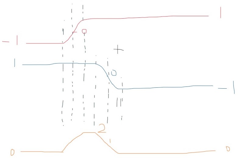
  23. “To make the noise proportional to the signal amplitude, we inject it directly in the µ-law domain.”

  24. “we find that by adding the noise as shown in Fig. 2, the network effectively learns to minimize the error in the signal domain”

  25. “we add noise … as suggested in [6]. … [6] Z. Jin, … ‘FFTNet: Areal-time speaker-dependent neural vocoder.’”

  26. “The simplifications above essentially make the computational cost of all the non-recurrent inputs to the main GRU negligible” from the paper

Windows AudioGraph

オーディオの入出力・ルーティング・処理を担うWinRT高レベルAPIs1.

入出力のマイク・ファイル指定、合成音の入力化などが可能.
UnityやWebにあるノードベースオーディオとだいたい同じ機能を提供.
音響効果の差し込みも可能.

Audio graphs - UWP applications | Microsoft Docs

WASAPIとの対比

  • shared/exclusive: shared-modeのみ.
  • 音響効果: callback (event-driven) モードで動作. AudioEffectオブジェクトに効果を実装し、Graph生成時にノードへeffectsを差し込む.
  • ファイル入出力: AudioGraphはデフォルトサポート.
  • 優先度制御: ベストの形を暗示的に提供. 高レベルAPIらしくてgood

AudioEffect

ノードへアタッチされ状態を持ち、packet処理ごとにcallbackで呼び出される音響効果.
IAudioEffectDefinitionを実装し、ON/OFFの制御が可能.
状態を持てるので1秒遅れエコーの実装等が可能.

Quantum/Buffer

Quantum: 1度に処理されるサンプル集合.
デフォルトで10msec分, DesiredSamplesPerQuantumで希望値設定可能.
AudioGraphのSamplesPerQuantumで現在値確認.
バッファサイズは直接指定がない. SamplesPerQuantum分のバッファで、毎回フルサイズ転送してると思われる.


  1. “This section provides detailed information about the Windows Runtime (WinRT) APIs. … Windows.Media.Audio” Windows Developer. Windows UWP Namespaces